Methods
Summary
Research region:
We are carrying out the experiment in the Reserve of the Hunting and Fishing Club Itororó, city of Uberlândia, state of Minas Gerais, southeastern Brazil (18°59' S, 48°18' W) (Figure 1 and 2). The reserve compasses an area of 6.4 km² of many types of Cerrado (i. e., Brazilian savannah) physiognomy (Figure 3).
The experiment will be carried out in Itororó reserve from March to June of 2017 (i.e., summer ending/fall beginning). Differently from most spiders in temperate regions, which have a clear seasonal cycle, adult females of species Argiope argentata in tropical regions are present throughout the year. Indeed, there is even an endemic Argiope species from Brazilian Cerrado called A. legionis, whose adult females are found between March and June. So, the period in which we are carrying out the experiments suits our goal, as we can count on the presence of adult females (which produce the most conspicuous web decorations/stabilimenta) in the research region.
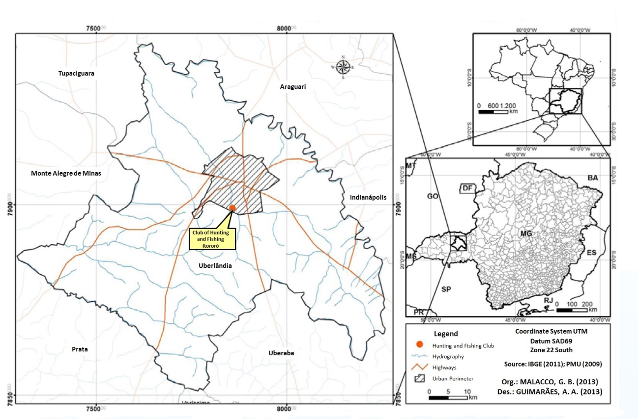
Figure 1: Location of the study area in Uberlândia city, state of Minas Gerais, southeastern Brazil.
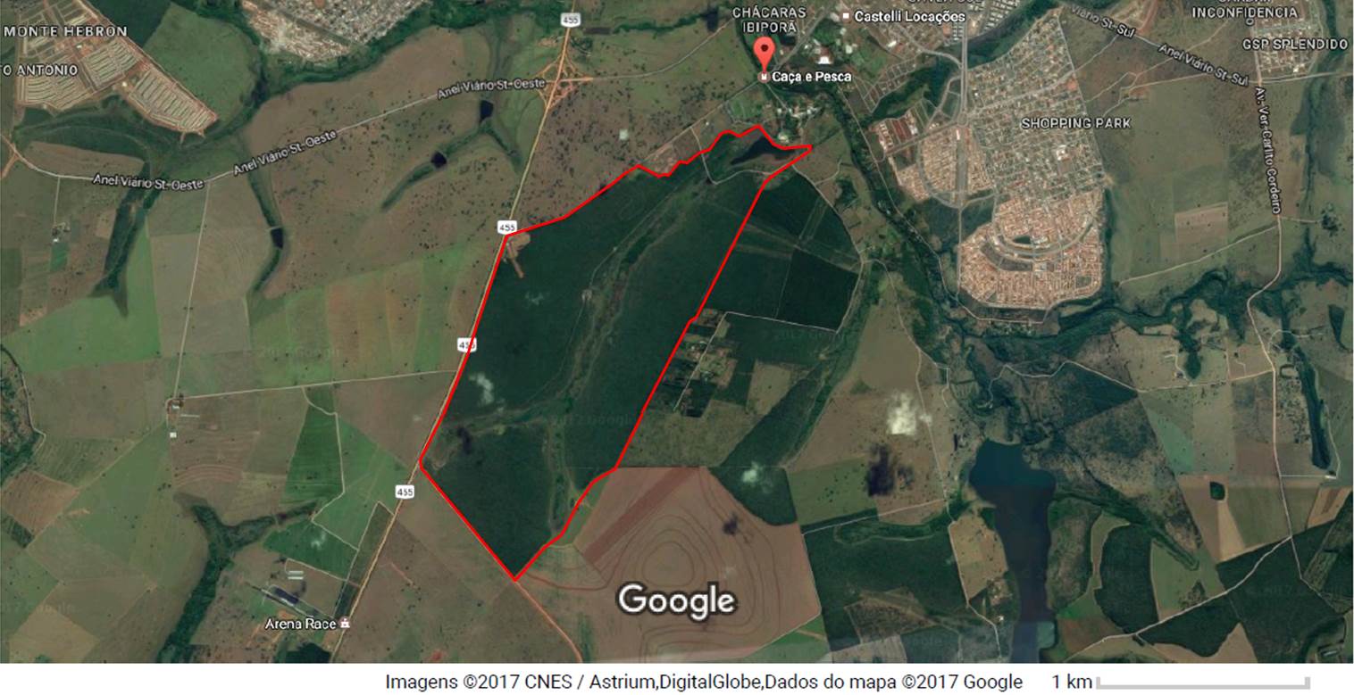
Figura 2: the Reserve of the Hunting and Fishing Club Itororó (perimeter highlighted in red).
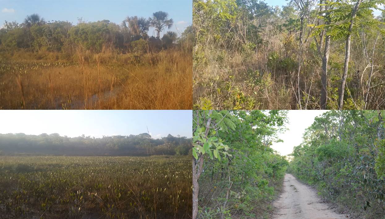
Figure 3: Different Brazilian Cerrado physiognomies in the Reserve of the Hunting and Fishing Club Itororó, Uberlândia, Minas Gerais.
Materials:
(1) Spiders: we are simulating the spider body with models made of wax-based plasticine clay (Figure 4). Plasticine clay models have become popular in experimental ecology. Usually, plasticine replicas of animals, such as larvae, frogs, and snakes, are placed in the field and examined for traits of physical attacks, like bites.
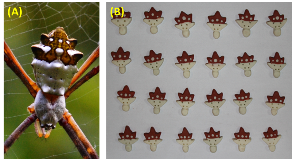
Figura 4: (A) A close-up of the body of an adult female from Argiope argentata species. (B) Models of A. argentata body made of plasticine clay.
(2) Webs/Sticky Traps: we are simulating Argiope spider webs with circular structures made of transparent acrylic glass. The circle is 25 cm in diameter, a size that is within the range of Argiope's web size (Figure 5). We also added two small perforations to the circular acrylic sheets for the passage of screws (Figure 5). This allows us to securely fasten the circular acrylic sheet to supporting stakes in the field. When placed in the field, we will spread entomological glue (Colly Química, Mombuca, São Paulo), which is insoluble in water, colorless and odorless, on the acrylic sheets to produce sticky trap for insects (Figure 6).
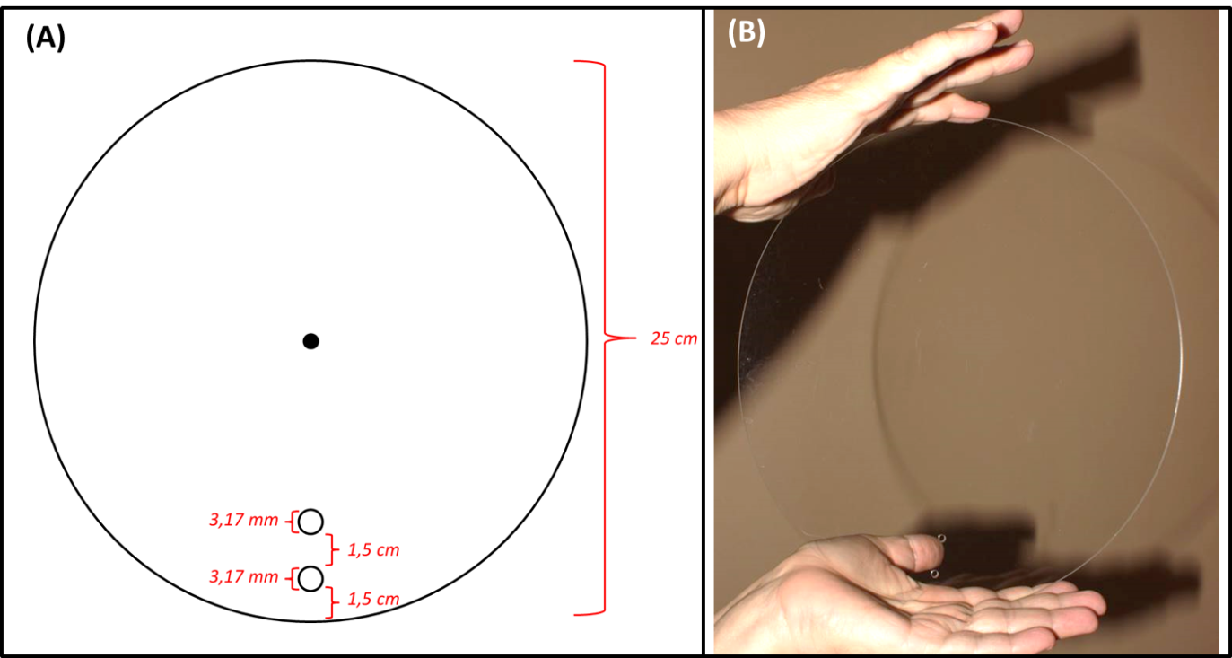
Figura 5: (A) Schematic drawing of the acrylic sheet used to simulate an Argiope web. The two small holes on the bottom of the sheet are used for the passage of screws, which fastens the sheet to supporting stakes in the field. (B) A picture of the circular sheet of acrylic glass used to simulate an Argiope web.
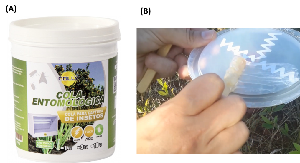
Figure 6: (A) Entomological glue; (B) Spreading of the entomological glue for manufacturing of sticky traps for insects.
(2) Stabilimenta (i.e., web decorations): we are simulating stabilimenta by using a brand of bond white paper (Grammage 120 g/m²) with high levels of UV reflectance. We processed the paper by laser cutting in shapes based on discoid and zigzag stabilimenta (Figure 7).
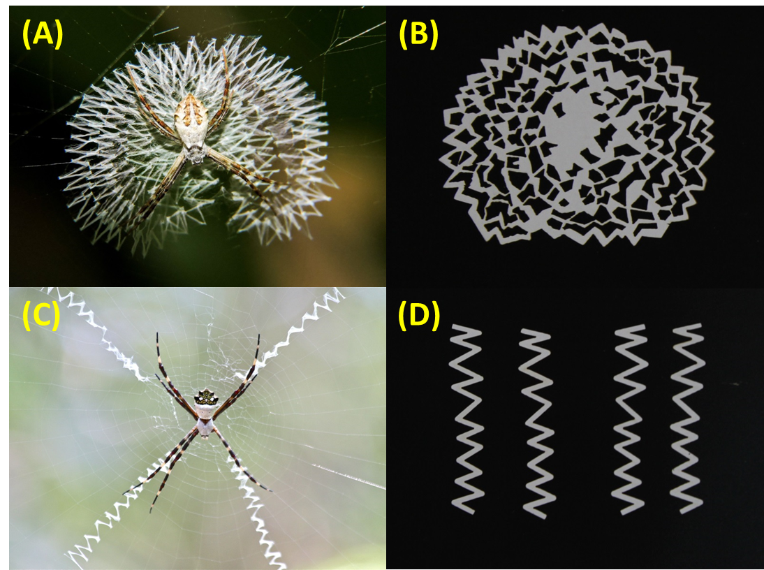
Figura 7: (A) Juvenile Argiope sp. with a discoid stabilimenta (Photo by Cheryl Harleston, from iNaturalist.org Creative Commons, Location: Yelapa, Jalisco, Mexico); (B) Simulacrum of a discoid stabilimenta made of UV reflective bond paper for our experimental purposes; (C) Female of Argiope argentata with zigzag stabilimenta (Photo by Laura Gaudette, from iNaturalist.org Creative Commons, Location: Fern Forest Nature Center, Florida, USA); (D) Simulacrum of a zigzag stabilimenta made of UV reflective bond paper for our experimental purposes.
(3) Ultraviolet absorbers: we selectively applied ultraviolet absorbers on our stabilimenta models to experimentally manipulate their UV reflection properties (Figure 8). We used the following chemical composition for the UV absorber solution: (1) Ethylhexyl Salicylate 5%, an absorber of UVB wavelengths; (2) Isoamyl p-Methoxycinnamate 10%, an absorber of UVB and short-wave UVA; (3) Menthyl Anthranilate 5%, an absorber of UVA; (4) Propylparaben 0.15%, a pharmaceutical preservative; (5) Mineral oil 100ml QS as a solvent. All these five substances are colorless and odorless, which prevents confounding variables in the experiment (Figure 8). Once the solution of UV absorbers was applied on the stabilimenta models, it effectively blocked a wide range of UV wavelengths spectra.
Furthermore, we also used a solution of only mineral oil and propylparaben 0.15% (i.e., excluding the UV absorbers) on the stabilimenta that we want to keep the UV reflectance properties. This allowed us to control for any confound effects of the substances used in the solution of UV absorbers; as well as the effect of oil on the paper used to make the stabilimenta models, since all the UV absorbers cited are oily substances.
Indeed, oily substances (such as the UV absorbers) reduced by around 50% the general reflectance of the bond paper used for making the stabilimenta, as the oiliness reduces the paper opacity. To minimize this issue, we are using a double layer of stabilimenta, in which a raw stabilimenta (i.e., without any treatment and, consequently, with intact reflectance properties) is completely overlaid by a exact shape stabilimenta with treatment (i.e., with UV absorbers solution or pure mineral oil). The superimposed stabilimenta recovered the original reflectance of the paper but also allowed us to block UV reflectance in selected stabilimenta, as the treated stabilimenta were external to the raw ones (see Figure 9 for more details).
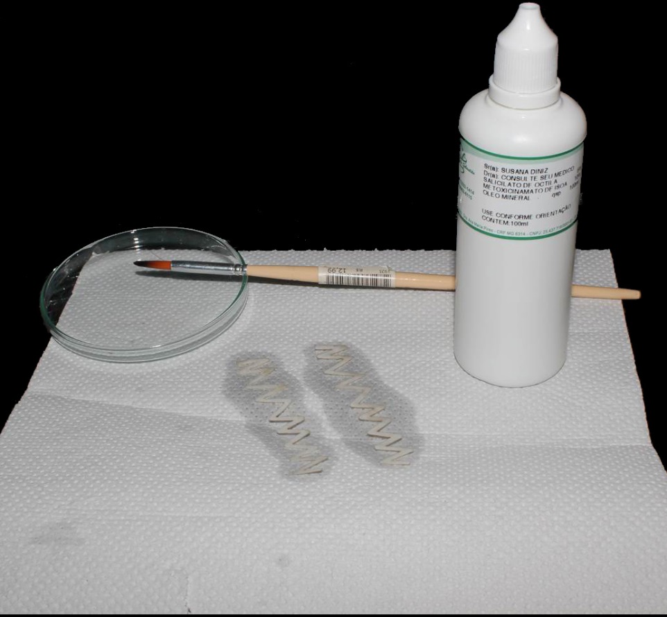
Figure 8: Solution of UV absorbers applied on zigzag stabilimenta models. Note that the solution is colorless.
(4) Transparent PVC film: we used sheets of transparent polyvinyl chloride (PVC) to put together all the components (i.e., the acrylic sheet, raw stabilimenta, treated stabilimenta and entomological glue) that formed our web model with stabilimenta. The PCV film has a good adherence to the acrylic, which dismissed the use of any adhesive substance to attach the stabilimenta on the acrylic sheet. See Figure 9 for a schematic illustration of the procedure to set up the web model of an Argiope spider.
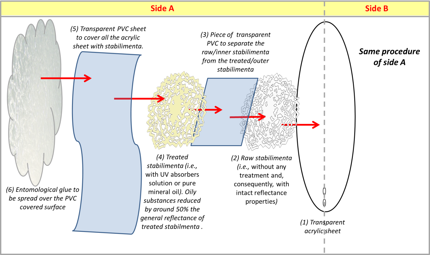
Figure 9: Schematic illustration showing the steps for setting up our experimental simulation of a spider web with stabilimenta (i.e., web decoration).
Experimental Treatments and Variables:
In order to better understand the role of the ultra-violet (UV) reflectance in different kinds of web decoration (also called stabilimenta) on prey attraction and predator attack, we are performing a manipulative experiment by simulating the spider web and their decorations. Experiments usually consists in two types variables: (1) explanatory variables (also called independent variables) are traits or factors that we think influence or direct the response variables; (2) response variables (also called dependent variables) are traits we think are influenced or shaped by the explanatory variables.
So, as explanatory variables, our experiment includes two crossed factors: (1) presence/absence UV reflectance, (2) stabilimenta type. The latter factor includes four levels:
(1) No stabilimenta:
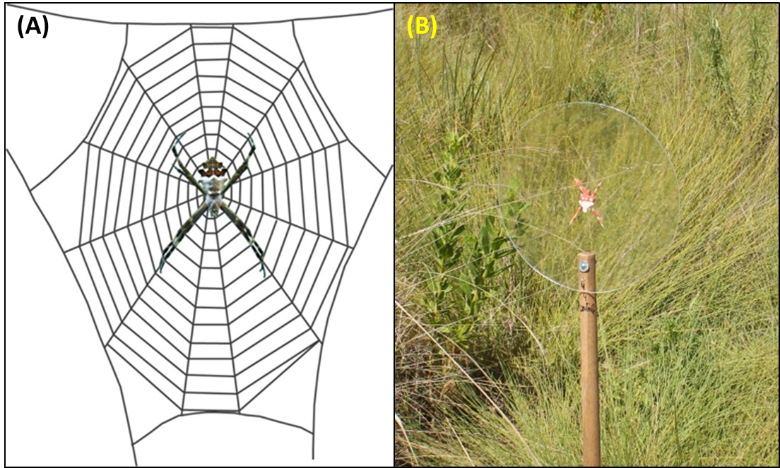
Figure 10: (A) Schematic drawing of an Argiope web without stabilimenta; (B) Web (without stabilimenta) and spider models placed in the field.
(2) Discoid:
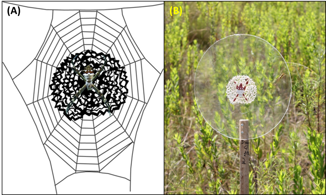
Figure 11: (A) Schematic drawing of an Argiope web with discoid stabilimenta. (B) Web (with discoid stabilimenta) and spider models placed in the field.
(3) Cruciate:
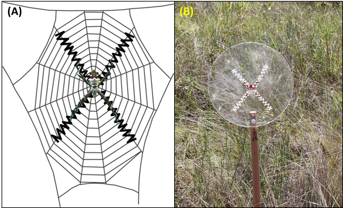
Figure 12: (A) Schematic drawing of an Argiope web with cruciate stabilimenta. (B) Web (with cruciate stabilimenta) and spider models placed in field.
(4) Linear:
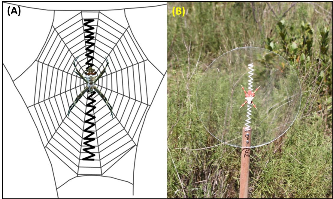
Figure 13: (A) Schematic drawing of an Argiope web with linear stabilimenta. (B) Web (with linear stabilimenta) and spider models placed in the field.
Summarizing, the experiment comprises a total of seven treatment levels: (1) no stabilimenta, (2) discoid stabilimenta with UV reflectance, (3) discoid without UV reflectance, (4) cruciate stabilimenta with UV reflectance, (5) cruciate without UV reflectance, (6) linear stabilimenta with UV reflectance, (7) linear without UV reflectance.
As response variables, our experiment includes measures of prey attraction and predator attack. Particularly, the prey attraction will be quantified as the number, diversity, and size of the intercepted prey by our web models (i.e., sticky traps). The prey attack will be quantified as the presence/absence of attack signs on our spider models.
Experimental Design:
Due to temporal and spatial heterogeneity, we opted for a randomized block design for the experiment. Blocks are a useful device to exclude biases due to specific local and temporal conditions of the environment. For instance, in Figure 14 you can see a common sight of the Brazilian savannah called Cerrado. In the same environment, there are different microclimatic conditions. For example, an experiment at position (A) (red arrow, Figure 14), which has higher tree density, would be less exposed to direct sun light than one positioned at (C) (blue arrow, Figure 14), which is an open grassy place. On the other hand, at position (B) (yellow arrow, Figure 14) there is a swampy-like water accumulation. So, an experiment positioned at (B) would be under high humidity conditions than experiments at (A) or (C).
In order to minimize the effects of environmental heterogeneity, blocks are designed to have relatively homogenous conditions inside, although these same conditions could vary greatly among them. Each block must have one replicate of all the experimental treatments. In the case of Figure 14, a researcher intending to do an experimental block design should first establish plots at positions (A), (B) and (C). The plots would be the embodiment of the idea of “blocks”. The size and location of these plots should be such that the local environmental conditions must be relatively similar inside the plot but heterogeneous among the plots. The research should then carry out a complete experimental trial inside each plot. In this way, the specific environmental conditions of each plot/block affect uniformly all the experimental treatments, which eventually allows the research to rule out biases due to environmental heterogeneity in the the case of any significant differences among experimental treatments. It is also important to remember that blocks are not only applied to spatial heterogeneity, but also to temporal variability. So, instead of a “blocking” by plots in a field, a researcher could block an experiment by time units such as hours, days, months or years.
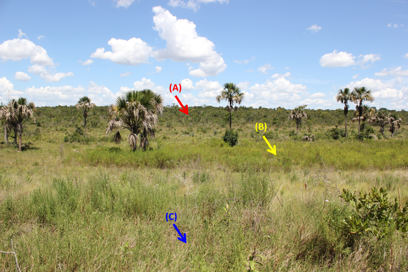
Figure 14: A Brazilian savannah (i.e., Cerrado) landscape showing heterogeneity in local environmental conditions, which is a source of uncontrolled variability in field experiments. For instance, at (A) there is a higher density of trees, what provides a more shaded environment than the open and grassy position at (C). At (B) there is a swamp-like water accumulation that creates more humid conditions, what is noticeable by the different plant composition of the vegetation patch pointed by the yellow arrow.
In our experiment, each block consists in a plot of 14 m by 14 m established in the field. In order to keep independency among plots, the minimum distance between any two plots is 100 m (Figure 15). We based this distance on previous research about flight distance of insects, in special the pollinating ones such as bees.
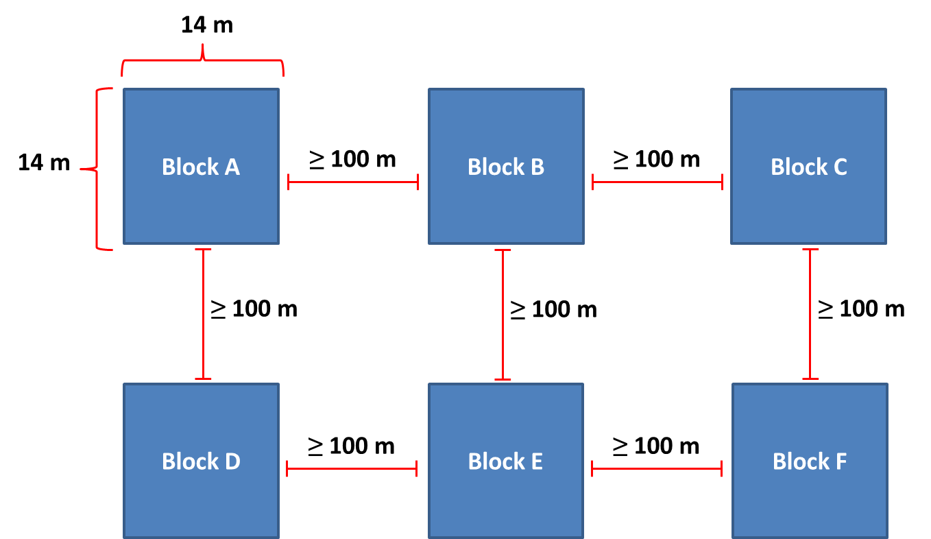
Figure 15: Experimental block design. Each block consists of a 14 m X 14 m plot placed in the field. In order to keep independency among the blocks, the distance between any two plots in at minimum of 100 m.
Each block has one replicate of the seven experimental treatments. The position of each treatment inside the plot is randomly assigned (Figure 16). In order to keep independence among the treatments inside each block, the minimum distance between any two treatments in the plot is 5 m (Figure 16). We based this distance on previous research about territorial distance among web spiders.
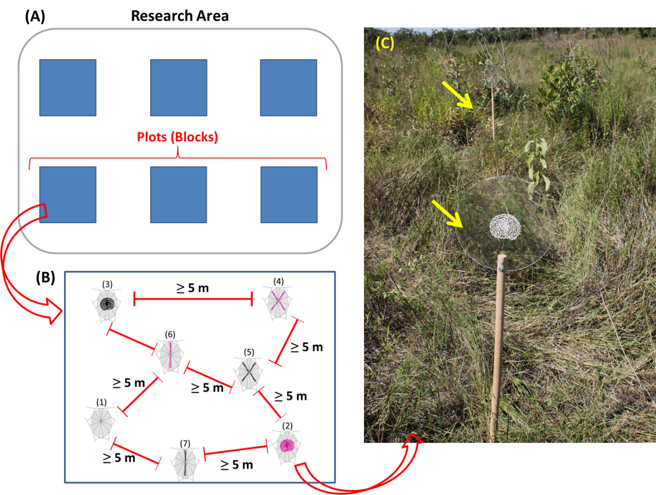
Figure 16: (A) Research area with sampling blocks (i.e., blocks). (B) A block showing one replicate of each experimental treatments: (1) no stabilimenta, (2) discoid stabilimenta with UV reflectance, (3) discoid without UV reflectance, (4) cruciate stabilimenta with UV reflectance, (5) cruciate without UV reflectance, (6) linear stabilimenta with UV reflectance, (7) linear without UV reflectance. Note the minimum distance of five meters among the experimental treatments and the randomly assigned position of each one. (C) A photograph illustrating two of the experimental treatments (yellow arrows) in a plot (i.e., block) in the field.
Our final goal is to accomplish a total of 16 up to 20 blocks, which would be a suitable sampling size for statistical analysis. However, the amount of field work impaired us to carry out all the blocks simultaneously. Therefore, we are carrying out two blocks for each field trip, which are usually one or two per week. This will lead to a temporally structured data sampling, which will be dealt as temporal data blocking. After the experiment setting, we wait a period of 48 h for collecting the samplings in the field and transport them to the laboratory for quantification and identification of the prey intercepted by the sticky traps.
Data Analysis:
Since the experimental designed in blocks, both temporally and spatially, we opted for mixed modeling for statistical analysis. Mixed models owe their name to the fact that they contain two types of explanatory variables:(1) Fixed factors: they are the explanatory variables of interest that the researcher deliberately manipulates. So, their variability fixed and controlled by the researcher. In this experiment, we have two fixed factors: the type of stabilimenta (i.e., no stabilimenta, discoid, cruciate and linear) and the presence/absence of UV reflectance.
(2) Random factors: they are also explanatory variables. However, differently from fixed factors, random factors are not controlled or of interest by the researcher. While the variability of fixed factors is previously established by the researcher, the random factor variability factor is wide and unknown, which eventually would become a noise in the data set. So, this random variability is taken into consideration in mixed models to avoid this noise, which improves the detection of effects from fixed factors. In this experiment, we include as random factors the plot (spatial heterogeneity) and the day when the experiment was carried out (temporal heterogeneity).
Protocols
This project has not yet shared any protocols.